Neural Net

Python

Let’s begin with the constructor method:

def __init__(self, layer_sizes, learning_rate=0.01, max_epochs=1000, batch_size=20):
    self.layer_sizes = layer_sizes
    self.learning_rate = learning_rate
    self.max_epochs = max_epochs
    self.batch_size = batch_size
    self.num_layers = len(layer_sizes) - 1
    # weights and biases initialization (He initialization)
    self.weights = [np.random.randn(layer_sizes[i], layer_sizes[i+1]) * np.sqrt(4.
        / (layer_sizes[i] + layer_sizes[i+1])) for i in range(self.num_layers)]
    self.biases = [np.zeros((1, layer_sizes[i+1])) for i in range(self.num_layers)]
    # cache for storing activations and inputs
    self.cache = {}

Here, layer_sizes is a list of integers representing the number of neurons in each layer of the network. The weights are initialized using the He initialization method, and the biases are initialized to zero. The cache dictionary is used to store the activations and inputs of each layer during forward and backward propagation. I was following Simon Prince’s explanation of neural networks from his new book, Understanding Deep Learning.

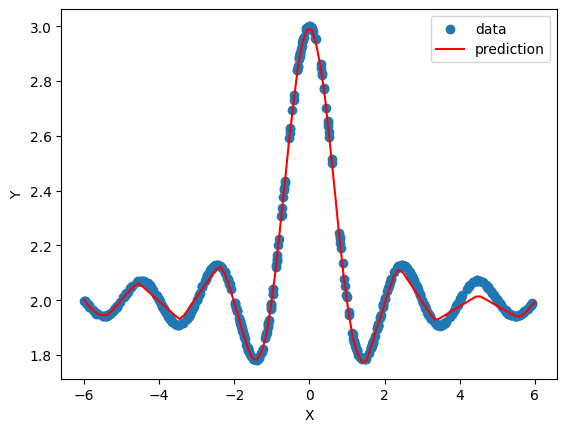
Interestingly, I had a learning moment here because initially, my implementation was for a shallow network with hard-coded layer sizes, and I had also left out biases to begin with (thinking that I would simplify the development experience). Boy, was I wrong. After an embarassingly long time of testing and not realizing what was wrong with my implementation, it finally dawned on me that the function I was trying to fit to, a sinc(x) function, never crossed the origin, and there was no way for my neural network to fit to a function that never crosses the origin without biases, which allow for affine transformations.

Forward propagation:

def forward_propagation(self, x):
    self.cache['a0'] = x
    for i in range(self.num_layers):
        z = self.cache[f'a{i}'] @ self.weights[i] + self.biases[i]
        self.cache[f'z{i+1}'] = z
        self.cache[f'a{i+1}'] = self.relu(z) if i < self.num_layers - 1 else z
    return self.cache[f'a{self.num_layers}']

Here, x is the input to the network, and the forward propagation method computes the activations of each layer using the ReLU activation function. The activations and inputs of each layer are stored in the cache dictionary for use in the backward propagation step.

Backward propagation:

def backpropagate(self, y):
    deltas = [None] * self.num_layers
    grads_w = [None] * self.num_layers
    grads_b = [None] * self.num_layers

    # Output layer error
    deltas[-1] = self.cache[f'a{self.num_layers}'] - y
    grads_w[-1] = self.cache[f'a{self.num_layers-1}'].T @ deltas[-1]
    grads_b[-1] = np.sum(deltas[-1], axis=0, keepdims=True)

    for i in range(self.num_layers - 2, -1, -1):
        deltas[i] = (deltas[i+1] @ self.weights[i+1].T)
            * self.relu(self.cache[f'z{i+1}'], derivative=True)
        grads_w[i] = self.cache[f'a{i}'].T @ deltas[i]
        grads_b[i] = np.sum(deltas[i], axis=0, keepdims=True)

    return grads_w, grads_b

The backpropagate method computes the gradients of the loss function with respect to the weights and biases of each layer using the chain rule. The deltas represent the error of each layer, and the gradients are computed using the activations and deltas of each layer stored in the cache dictionary.

One step of stochastic gradient descent:

def stochastic_gradient_descent_step(self, grads_w, grads_b):
    for i in range(self.num_layers):
        self.weights[i] -= self.learning_rate * grads_w[i] / self.batch_size
        self.biases[i] -= self.learning_rate * grads_b[i] / self.batch_size

In this method, the weights and biases of each layer are updated using the gradients computed in the backpropagation step. The learning rate and batch size are used to scale the gradients.

Helper function to compute loss during training:

def compute_loss(self, y, y_hat):
    loss = np.mean((y_hat - y)**2)
    return loss

Helper functions for calling forward propagation and for ReLu activation:

def predict(self, X):
    return self.forward_propagation(X)

def relu(self, x, derivative=False):
    if derivative:
        return np.where(x > 0, 1, 0)
    return np.maximum(0, x)

Finally, the training loop:

def fit(self, X, y, X_val=None, y_val=None, get_validation_loss=False):
    training_loss = []
    if get_validation_loss:
        validation_loss = []
    n_samples = X.shape[0]
    n_batches = n_samples // self.batch_size

    for epoch in range(self.max_epochs):
        indices = np.arange(n_samples)
        np.random.shuffle(indices)
        X_shuffled = X[indices]
        y_shuffled = y[indices]

        for batch in range(n_batches):
            start = batch * self.batch_size
            end = start + self.batch_size
            X_batch = X_shuffled[start:end]
            y_batch = y_shuffled[start:end]

            y_hat = self.forward_propagation(X_batch)
            loss = self.compute_loss(y_batch, y_hat)
            grads_w, grads_b = self.backpropagate(y_batch)
            self.stochastic_gradient_descent_step(grads_w, grads_b)
            training_loss.append(loss)

            if get_validation_loss:
                X_val_batch = X_val[start:end]
                y_val_batch = y_val[start:end]
                y_val_hat = self.forward_propagation(X_val_batch)
                val_loss = self.compute_loss(y_val_batch, y_val_hat)
                validation_loss.append(val_loss)

        if epoch % 100 == 0:
            print(f'Epoch {epoch}, Loss: {loss}')

    if get_validation_loss:
        return training_loss, validation_loss
    return training_loss

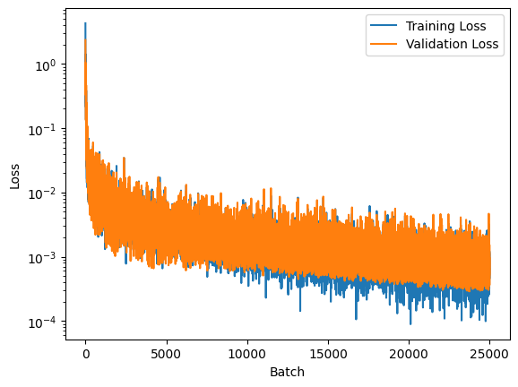
In the training loop, the training data is shuffled at the beginning of each epoch, and the network is trained using mini-batches of data. The loss is computed for each batch, and the gradients are computed using backpropagation. The weights and biases are updated using stochastic gradient descent. If the validation data is provided, the loss is computed for the validation data as well.

I chose the sinc(x) function to test my network— I wrote a brief script and used Numpy to generate a noisy dataset with just 500 samples. Fitting actually worked out quite well, despite not having implemented the Adam solver:

layer_sizes = [1, 50, 50, 50, 50, 50, 50, 50, 50, 50, 1]
 smol = smol_brain(layer_sizes=layer_sizes, learning_rate=0.01, max_epochs=1000, batch_size=20)
 training_loss, validation_loss = smol.fit(x_train, y_train, x_val, y_val, get_validation_loss=True)

Mojo

Mojo implementation writeup in progress.